Forecasting Next Week's Kale With 180 Data Points: Where Machine Learning Helps a 38-Producer Co-op, and Where a Moving Average Wins

How much data does a 38-producer co-op actually have?

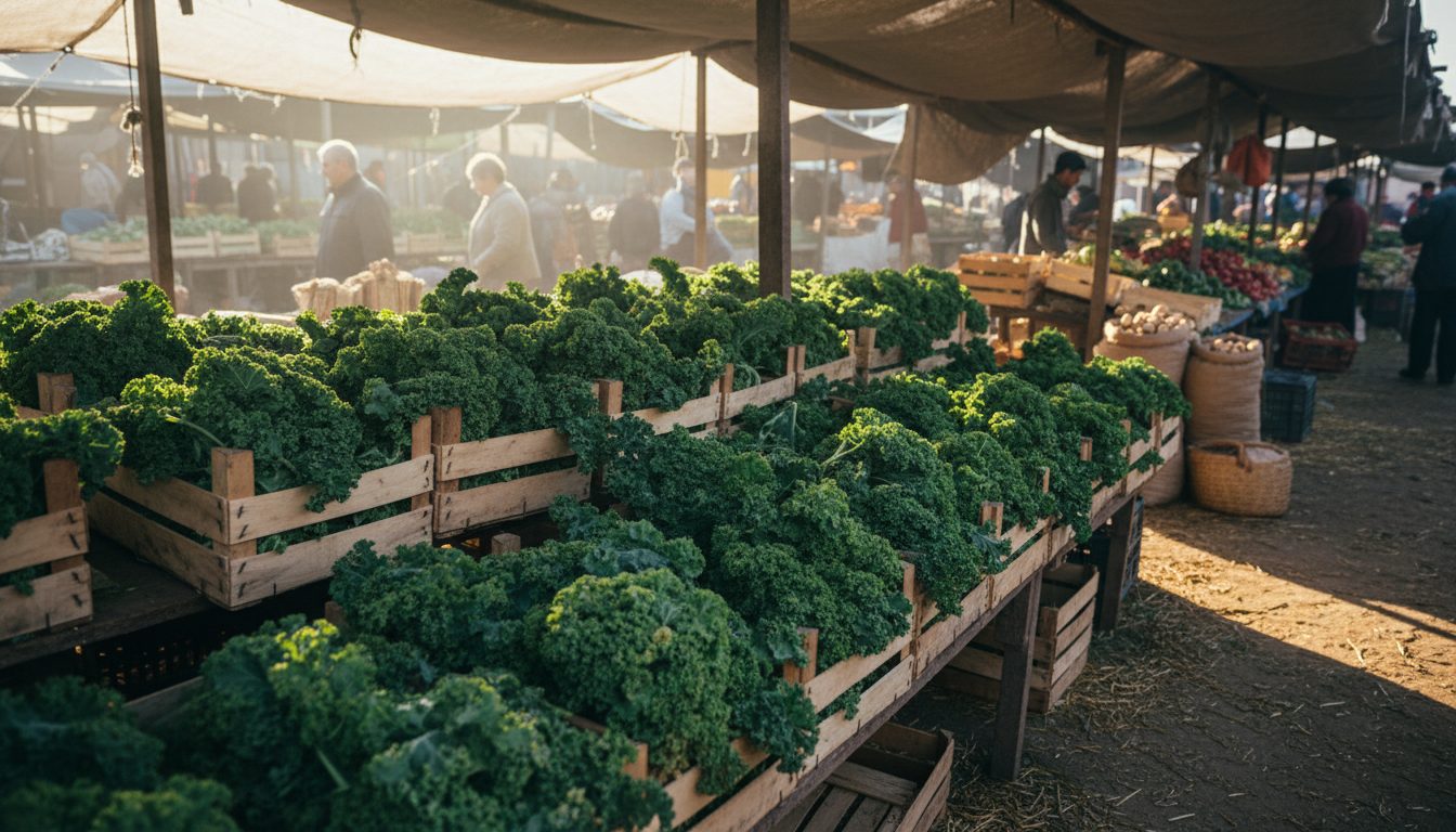
A weekly co-op with 38 producers and two years of trading has roughly 100 weekly cycles, and for any single product perhaps 60 to 90 weeks where that product was even available. Kale sold across 12 autumn and winter weeks a year gives you around 24 observations, not thousands.

The number in the title is generous. Take one product, one channel, one co-op: kale, home delivery boxes, weekly ordering window. Two seasons of trading might produce 180 order lines in total, spread across perhaps 24 sales weeks and 90 distinct shoppers. That is the entire training set. Aggregate to the level you actually need to forecast, which is kilograms of kale to request from producers for next week, and you have 24 numbers.

This matters because almost every published guide to AI demand forecasting assumes the opposite problem. Those articles are written for a distributor with 400 SKUs, five depots and six years of daily transactions, where the challenge is compute and feature engineering. In a short food supply chain the challenge is that half your products have fewer observations than a school science experiment, and the ones with more observations have their seasonality baked in so hard that a model can memorise the calendar and learn nothing else.

Where a three-week moving average wins

For any product with a stable weekly rhythm and no strong trend, a three-week moving average of recent sales, adjusted by hand for known events, beats a trained model on small local data. It is transparent, needs no maintenance, survives missing weeks, and fails in ways an administrator can see and correct.

The reason is variance. With 24 observations and 10 candidate features, a model will fit noise and present it with a confidence the data does not support. A moving average makes one assumption, that next week resembles the last three, and that assumption is correct most of the time in a weekly delivery co-op with a repeat shopper base. Where it is wrong, it is wrong by a small, bounded amount.

Simple statistics are the right tool in most of the cases a co-op administrator faces week to week.

Products with fewer than roughly 20 sales weeks of history: there is nothing for a model to learn that a human cannot read off a chart.
Products with flat demand and high repeat purchase, such as eggs, potatoes, bread and milk: the previous three weeks are close to a perfect predictor.
A brand new producer or a new product: no history at all, so use a comparable product's curve and a conservative first-week quantity.
One-off shocks such as a heatwave, a road closure or a festival: judgement plus a manual override beats any historical pattern.
Anything where the cost of being wrong is low: if unsold bunches go to the co-op's own market stall, precision has little value.

Where prediction genuinely helps on small local data

Machine learning earns its place in a short food supply chain not on total demand but on structure: which shoppers are about to lapse, which order lines a shopper reliably repeats, which weeks a seasonal product will peak, and which producer declarations habitually overstate what arrives. These have more observations per prediction than product-level demand does.

The trick is to change the unit of analysis. Forecasting kilograms of kale gives you 24 rows. Forecasting whether a given shopper will order kale next week, given their last eight weeks of baskets, gives you 90 shoppers times 24 weeks, which is over 2,000 rows with genuine variation in it. Shopper-level repeat prediction is a small-data-friendly problem because the panel is wide even when it is short. Summing individual probabilities then gives you a demand estimate that carries an honest confidence interval, because you know how many shoppers it rests on.

The same shift works elsewhere. Declaration reliability is a per-producer, per-week problem with hundreds of observations across the co-op, so a simple model can learn that producer 14's leafy greens arrive at 85 percent of declared weight in July and 100 percent in October. Basket completion, delivery failure risk and slot demand all have similar shapes: many small events rather than few big aggregates.

Which signals matter in a short food supply chain

Five signal families carry almost all the predictive power in local food demand: calendar position in the growing season, weather in the ordering window, holiday and school weeks, repeat shopper cohort behaviour, and catalogue composition, meaning what else was available to order that week. Everything else is usually noise at this data volume.

Season is not a smooth sine wave here. It is a set of hard on/off gates: the first week tomatoes appear, the week strawberries end, the week the co-op's only kale grower starts cutting. A model that treats week-of-year as a continuous feature will smooth across those edges and be confidently wrong at exactly the transitions that matter. Encoding availability windows explicitly, per product per producer, does more than any algorithm choice.

Weather works differently from the industrial case too. It affects supply through the producer's field, and it affects demand through the shopper's cooking plans, often in opposite directions in the same week. A cold snap raises soup vegetable orders and slows growth in the tunnel. Catalogue composition is the signal most co-ops forget: kale sales drop when chard, spinach and cabbage all appear the same week, so a kale forecast that ignores substitution will over-order every time the greens overlap.

Season and availability windows: explicit per-product start and end weeks, not a continuous week-of-year term.
Weather: temperature and rain during the ordering window, with separate treatment of the supply effect and the demand effect.
Calendar events: public holidays, school terms, local festivals, and the week before and after each.
Cohort behaviour: weeks since a shopper joined, purchase frequency, and whether they are in their first four orders or their fortieth.
Catalogue composition: how many substitute products were listed that week, and at what price relative to each other.

A practical forecasting ladder for a co-op

Start with a moving average, add manual overrides, then add seasonal adjustment, then add shopper-level repeat probability, and only then consider a trained model. Each rung should be shipped and used before the next is built, because each one absorbs error the next rung would otherwise be asked to explain.

In practice most co-ops should stop at rung three or four for a long time. Rung one costs an afternoon of SQL. Rung two is a text box next to a number in the admin interface, plus a habit of using it. Rung three encodes availability windows and holiday weeks, which produces most of the accuracy gain a co-op will ever see from forecasting. Rung four is where the shopper-level panel comes in, and it is the first rung where anything deserving the label machine learning appears.

Measure honestly at each rung. Track mean absolute error in the unit the operation cares about, which is kilograms or units per product per week, and track it against the naive baseline of last week's sales. If a new rung does not beat the naive baseline by a margin larger than the week-to-week noise, it has not earned its place. Also track the asymmetry: over-ordering leafy greens costs waste and a producer credit note, while under-ordering costs a missing line in 40 boxes and an apology. A forecast that is unbiased in aggregate but wrong in the expensive direction is worse than a slightly biased one.

Rung 1: three-week moving average per product, shown next to the declaration screen.
Rung 2: administrator override with a required one-line reason, logged for later review.
Rung 3: seasonal gating and holiday-week multipliers derived from last year's same weeks.
Rung 4: shopper-level repeat probability summed to a product forecast with a confidence range.
Rung 5: a gradient-boosted or regularised regression model on the full signal set, evaluated against rung 4 before it is trusted.

How to tell a real forecast from a confident guess

A usable forecast in a short food supply chain states a range, names the number of observations behind it, and shows what it assumed. A number with no interval and no history count is a guess wearing a decimal point, and producers stop trusting it the first week it is badly wrong.

This is a product design problem more than a modelling one. If the admin interface says 42 kg of kale, an administrator will order 42 kg. If it says 34 to 50 kg, based on 19 comparable weeks, no kale sold in 3 of the last 8 weeks, the same administrator asks a producer a question and lands somewhere sensible. The interval is not a hedge, it is the information. On small-N data, honestly wide intervals are the correct output, and narrow ones should be treated as a bug.

The trust economy matters as much as the arithmetic. Producers plan cutting and harvest around what the co-op asks for, so a forecast that quietly over-asks pushes waste and cost onto the grower rather than the co-op. Any forecasting feature in local food should be introduced as a suggestion beside the human decision, never as an automatic order, and its historical accuracy per product should be visible to the people whose week it shapes.

Key Takeaways

A single product in a weekly co-op typically has 20 to 30 usable observations, not thousands, so most published AI forecasting advice does not transfer.
For flat, high-repeat products and anything with under about 20 sales weeks of history, a three-week moving average plus manual overrides beats a trained model.
Prediction pays off when you change the unit of analysis: shopper-level repeat probability, declaration reliability and slot demand have wide panels even on short histories.
The signals that matter locally are availability windows, ordering-window weather, holiday and school weeks, cohort age and catalogue substitution, not generic trend and price elasticity.
Always publish a range and the observation count, and measure every rung against the naive last-week baseline before trusting it.

The declaration data these forecasts depend on is described in our Tuesday night declaration post, which covers how producers post next week's availability and the rules that keep those numbers honest.

Frequently Asked Questions

Can you do demand forecasting with only one year of sales data?

Yes, but only at the coarsest level. One year gives you a single observation of each seasonal week, which is enough to gate availability windows and flag holiday weeks, but not enough to separate a real seasonal effect from one unusual week. For the first year, use a moving average for near-term quantities and treat last year's same week as a sanity check rather than a prediction.

What forecast accuracy should a small food co-op expect?

Judge accuracy relative to the naive baseline rather than against an absolute target. For stable staples like eggs and potatoes, a moving average often lands within 10 to 15 percent of actual weekly volume. For weather-sensitive leafy greens and soft fruit, errors of 30 percent or more are normal, which is why range-based forecasts and manual overrides matter more than model sophistication.

Is it worth buying an AI demand forecasting tool for a food hub?

Usually not as a separate purchase. Off-the-shelf forecasting tools expect long daily transaction histories and hundreds of stable SKUs, neither of which a food hub has. The higher-value investment is clean order-line and declaration data inside the platform you already run, plus simple baselines surfaced where decisions are made.

How do you forecast demand for a brand new product or producer?

Borrow a curve from the closest comparable product already in the catalogue, then start deliberately small. Order a conservative first-week quantity, watch the sell-through rate and the share of shoppers who add it, and adjust in the second and third weeks. After four or five weeks you have enough to switch to a moving average of its own history.

What is the difference between forecasting supply and forecasting demand in a short food supply chain?

Demand forecasting predicts what shoppers will order; supply forecasting predicts what producers will actually deliver against what they declared. Both are needed, because a co-op's real constraint is the smaller of the two. Supply-side prediction is often the easier win, since declaration versus delivered weight is recorded every week across all producers, giving far more observations than any single product's sales history.